On the last post I detailed all the ways we screwed up our magnetometer implementation. Here I’m going to talk about how we can make it better.
I knew from our previous analysis that low-pass filters couldn’t separate our signal out. But I suspected an FFT might.
Long explanation short, Fast Fourier Transforms can take a chunk of sampled data, and compute how much signal there is at various frequencies inside the data. Lets demonstrate.
Here is the signal I originally expected to see, as recreated in a simulation:

Ideal field strength plot
But as discussed in my previous post, the motor magnets add a lot of noise. Here’s what that probably looks like:

Simulation of motor noise
This looks pretty gnarly, and does resemble the plot of actual data from the previous post. The untrained eye might think it’s impossible to get our ideal signal out of this plot, but that’s not quite true. Here’s what we get when we take the FFT of this data:

FFT of the noisy data
In this simulation, the robot is spinning at 1500RPM or 25Hz. So we see a matching peak at 25Hz, that’s the signal we want. But the motor noise represents as a peak at 75Hz and 525Hz.
There is a third peak, but its frequency is too high to appear in this plot. We will generally only consider the first noise component anyways, as it is the strongest and hardest to separate.
Now, the thing about FFTs is that not only do they give you the magnitude of a frequency component, they can also give you the phase shift. And for us, the phase of that 25Hz signal is our heading measurement. So if we can take an FFT of our magnetometer data and find the first peak, we can get our heading measurement. How hard could it be!
Slowly Adding Reality
We have to consider that FFTs are very expensive (read: takes a lot CPU time), and we are running this on a relatively slow microcontroller. So we need to take some shortcuts to make our algorithm cheaper.
First, we will only computer over a narrow window of data. The fewer the samples, the less work you need to do to compute the FFT. The tradeoff is that you lose some resolution; instead of knowing your signal is at exactly 25Hz, you can only know that it’s somewhere between 24 and 26Hz, for example. But even at 32 samples we keep enough resolution to work with.
We will also reduce our sample rate to one our magnetometer can actually achieve. For the BMM150 that’s 300Hz.

More realistic FFT plot. Robot is spinning at 18Hz
Here you can see that resolution tradeoff in practice. That said, our signal of interest (SoI) is still easily discernible.
But Can we do it Cheaper?
The thing is, we don’t really care about the FFT results of any frequency that isn’t our SoI. If we knew in advance what frequency our SoI is, we could try to compete a partial FFT of just that bin.
Goertzel’s algorithm is exactly this. Pre-compute some parameters given your sample frequency and signal frequency, and you get an algorithm that can extremely efficiently find the magnitude and phase components of just your signal frequency.

Results of a Goertzel algorithm on simulated magnetometer data, constant speed
You can find my python Goertzel implementation here. I used these sims to generate all of the plots in this post.
I’m flippant about saying we have knowledge of our SoI’s frequency because the use of an accelerometer to measure rotation speed is already well understood. I don’t love adding a back a $10 chip (H3LIS331DL) that I spent years trying to replace. But it significantly reduces the computation requirements of our algorithm, and it’s also critical to counteract the effects of acceleration.
The Effects of Acceleration
A meltybrain spends most of its time in a match accelerating. If it’s at top speed, it should be getting busy smashing its opponent and accelerating again.
So lets adjust our sim to account for this and see how our algorithm performs.

Results from a naive Goertzel of accelerating data
Turns out it doesn’t do well at all. Here’s another view where I calculate the heading error across the sim.
Showing phase error over time for a naive Goertzel on accelerating data.
This occurs because our SoI no longer exists at one frequency. As the robot accelerates, it increases in frequency. Goertzel’s, and FFTs in general, calculate as if the components of a signal maintain the same frequency over the window of samples. If this isn’t true, you get artifacts that throw results off. Here’s what our FFT plot looks for this simulation.

FFT result of data with accelerating components
As you can see, there are now “phantom” signals all over the plot. These will disrupt the measurements of our real signals.
Resolving this problem requires us doing something a little weird.
Adaptive Sample Rate
We can lean on a unique advantage that we have to fix our acceleration problem. That being, an accelerometer that can provide us near real-time frequency measurements. The H3LIS331DL accelerometer can measure at 1KHz, roughly 3X the sample rate of our magnetometer. If our rotation speed is accelerating, we can see that immediately in the data. Additionally, the BMM150 can be triggered manually. More on that in a second.
Reminder: the Goertzel’s algorithm must be configured for a particular sample rate and target frequency. The way these parameters work, however, is if you double the target frequency and double the sample rate, Goertzel’s will give the same exact answer.
So if the accelerometer measures that the robot is spinning 5% faster, we can boost the magnetometer sample rate 5% to match. Doing so will ensure the Goertzel’s algorithm will continue giving good answers with exactly the same parameters.
We can think about this another way. By saying we are configuring Goertzel’s algorithm for a particular sample frequency, we are also saying we are configuring Goertzel’s for a particular sample period. As long as we ensure each sample represents the same percentage of a signal period, Goertzel’s will provide valid data.
We can lean on the accelerometer to predict how much of a signal period has elapsed since the last magnetometer measurement. If we are seeing a higher rotation speed, then we can predict that the signal period is elapsing faster. Every millisecond, we get a new accelerometer measurement that we can use to adjust our prediction. If we trigger a magnetometer measurement after exactly the correct amount of signal period every time, Goertzel’s will give us the correct data no matter how the frequency changes over the sample window.

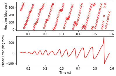
Simulation of a Goertzel’s algorithm with adaptive sample rate, in a dramatically decelerating scenario
Pictured above shows our “adaptive sample rate” in action. The robot quickly decelerates to half speed, but Goertzel’s stays roughly on track throughout. It accomplishes this by slowing down the magnetometer samples to match the decrease in SoI frequency (you can see the X’s become increasingly spread out in the plot)
That simulation is also a bit more advanced, in that it includes the effect of measurement error. We are effectively doing a discrete time integral of the accelerometer data, after all. Any error present will add up to an extent. However, it will not add up infinitely over time like it would if were trying to get position directly from our speed measurements. In our case, the error effectively “resets” every measurement. This has been a lot of words, so below is a graph that attempts to demonstrate how our adaptive sample rate helps.

Showing how rotation speed can be integrated to correct for acceleration in the Goertzel/FFT data
As an aside, you might wonder how the heading measurement can be useful given that the sample window now represents a variable amount of time. Especially since the heading measurement is relative to the first measurement in the window, so all of our measurements are 32 samples late! The trick is, if we are ensuring that each sample is relatively the same period apart, then the entire window has a relatively fixed phase shift from the first sample. And as discussed in previous posts, fixed phase shifts can be ignored because they will be adjusted manually regardless.
Lets see how this algorithm performs.

Heading error of an adaptive goertzel implementation in a rapidly decelerating environment
If the worst our heading error gets is 20°, we’ll take it.