Like the beacon in the post before, the accelerometer algorithm has some room to improve. The primary reason is the same as well: acceleration causes problems. And now, for the driest heading I have yet written on this blog:
What the algorithm does, in graphs
Like the improved beacon algorithm, there's really no better way to explain than with graphs. Here's what our bot is doing when it's spinning at a constant speed:
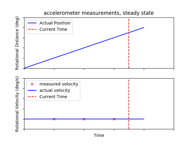
Revisiting our first-order algorithm for calculating our heading:
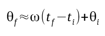
If we multiply the speed of the bot by how long it has been spinning that fast, we get how far it has spun. This is accurate so long as we are measuring infinitely fast, or so long as the robot continues spinning at the same speed.
Lets look at what happens when the robot accelerates:

This case causes our algorithm to generate lots of error. It's not obvious where the error comes from, so lets visualize what our algorithm is calculating:

The red shaded area above is comprised of three rectangles, one for each measurement. It's width is the distance in time, it's height is the measured speed. What our algorithm tries to do is calculate the size of the area under the velocity line. This area equates to the distance traveled.
The simplest algorithm uses rectangles because they are easy to calculate area for (It's also known as the Riemann Sum). You simply multiply length (measured velocity) by width (time interval). But the graph above shows that when the velocity changes over time, some area is missed by the rectangles. All missed area represents error in the measurement, which causes drift.
If we want to reduce the error in our measurement, we can do two things:
1. Measure faster
If we measure infinitely fast, there will be no error. Or for a more likely solution:
2. Change how we calculate area
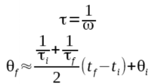
Instead of using rectangles, we can use a different shape that better matches our line. In the case above, the best match is a trapezoid, so we will use the trapezoidal rule here. The area of a trapezoid can be found with:
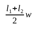
Where our trapezoid is defined as:

The final equation, part A:

Given that you run this equation every time you get a new accelerometer measurement, the variables marked "i" are from the previous measurement and the variables marked "f" are from the recent measurement.
However, this equation can only run every time we get a new accelerometer measurement. If our code runs faster than our accelerometer (which is likely), then we will need to guess at our rotational velocity in between measurements. We can do this by borrowing an equation from the beacon algorithm:
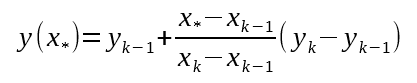
Remember this one? We can use it to extrapolate our current velocity given that we remember our last two measurements. Substituting in our variables:
The final equation, part B:
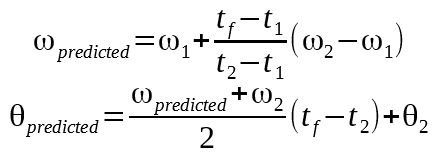
Where (ω_1, t_1) is the earliest measurement, (ω_2, t_2) is the most recent measurement, Θ_2 is the angle at the most recent measurement, t_f is the current time, and Θ_predicted is where we expect the bot is pointing now.
Practical Considerations
In my implementation, I wasn't able to use the equations above as-is. This is due to the limitations of embedded arithmetic.
Time in my bot is measured in microseconds, but distance is measured in degrees. so to bridge the gap, my velocity term needed to be in units of degrees per microsecond. In practice, that is a tiny number. A speed of one revolution per second is 0.00036 degrees per microsecond!
Our microcontroller doesn't have a floating point unit, so any floating point operations are emulated in software. Consequently, floating point operations will be very slow. To remedy this, we can try to minimize our use of floating point in favor of integer math.
Instead of running calculations using degrees per microsecond, we can use microseconds per degree. This turns our 0.00036 into 2777.78, which (rounded to 2777) is much faster to do math with.
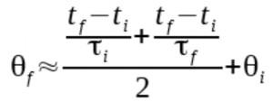
To support using inverse speed, however, we need to change our equations.
This doesn't help much on it's own, but we can move the equation around a bit
To explain why this equation works better, lets say that the robot is moving at a constant 1000 rpm (around where we expect to operate) and the accelerometer is being sampled at 100Hz.
1000 rpm equates to 166.67 us per deg, which as an integer rounds down to 166. This is tau.
t_f - t_i is the time between measurements in microseconds. At 100Hz, that time is 10ms, or 10,000us. 10000/166 = 60.2 degrees.
I was able to do all of this math with integers only without losing too much precision. That would be impossible without redefining the equation in this way. This method can be used for final equations part A and B similarly.
Conclusions and Caveats
These equations should present much less drift than previously. Like for the beacon algorithm, we can trade complexity for precision.
The main caveat here is that error is still generated whenever the acceleration changes. This should not cause as much of an effect as acceleration did on the rectangular method. But if you truly want the best-of-the-best here, you can substitute the trapezoidal method with Simpson's rule to account for when the acceleration varies over time.
And you're only going to be as accurate as your calibration. See my next post for how I calibrated my bot.
Thanks to teammate Novia Berriel for working out the math